


#commoncore Project Methodology
 This section provides a detailed discussion of the methods used to arrive at the conclusions in #commoncore: How social media is changing the politics of education. After describing how we retrieved the Twitter data, which was used in all sections of the website, we then detail the analyses for each of the five acts in the website.
Twitter Data
Twitter (http://www.twitter.com) is a free online global social network that combines elements of blogging, text messaging and broadcasting. Users write short messages limited to 140 characters, known as ‘tweets’, which are delivered to everyone who has chosen to follow the sender and receive their tweets. Within each tweet is possible to link to other media and to embed video, images and use searchable metadata named as hashtags (a word or a phrase prefixed with the symbol # as metadata).
Twitter users can interact and communicate in different ways and users are finding new and creative ways to get the most out of each tweet. First, they can write simple messages called tweets adding images, videos, hashtags, etc. Second, tweets can be further disseminated when recipients repost them through their timeline. This technique, called retweeting, refers to the verbatim forwarding of another user’s tweet. A third type of messaging is a variant of tweeting and retweeting, called mentioning. Mentions include a reference to another Twitter user’s username, also called a handle, denoted by the use of the “@” symbol. Mentions can occur anywhere within a tweet, signaling attention or referring to that particular Twitter user.
To collect data on keywords related to the Common Core we utilized a customized data collection tool developed by two of our co-authors, Miguel del Fresno and Alan J. Daly, called Social Runner LabTM. Social Runner LabTM allowed us to download data in real time directly from Twitter’s Application Programming Interface (API) based on tweets using specified keywords, keyphrases, or hashtags. We bounded the data collection to a set of keywords and captured Twitter profile names as well as the tweets, retweets, and mentions posted. Our data include messages that are public on twitter, but not private messages between individuals, nor from accounts which users have made private or direct messages.
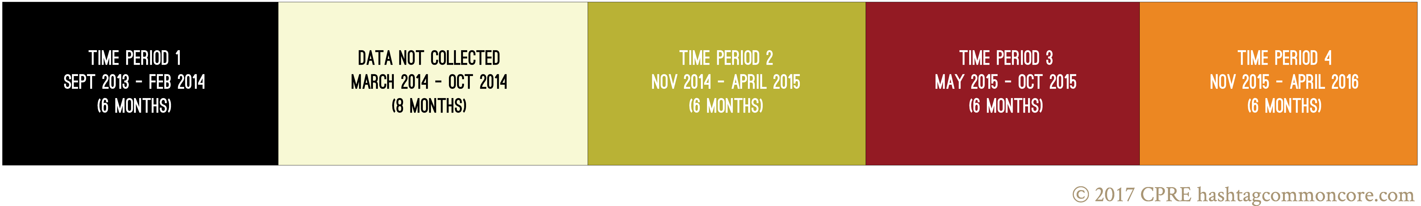
In the data collection for the first six months of our study, we collected only tweets that used commoncore. In the last 18 months of our data collection we added ccss and stopcommoncore to our collection dataset. Thus, as can be seen in Figure 1, we collected data for 24 months over the period from September 2014 to April 2016. For the sake of comparability, we broke our data into six-month periods. For more details about the data, see The Dataset in Act 1.
The analysis that produced the conclusions of each Act in the website used different segments of the Twitter dataset and employed distinct methods. Table 1 shows a summary of the data used for the analysis conducted for each Act, as well as the samples of actors and tweets, the keywords, and the methods that were utilized.
Figure 1. Time Periods Analyzed in #commoncore study
The analysis that produced the conclusions of each Act in the website used different segments of the Twitter dataset and employed distinct methods. Table 1 shows a summary of the data used for the analysis conducted for each Act, as well as the samples of actors and tweets, the keywords, and the methods that were utilized.
Table 1. Data and Method for Each Act of the #commoncore website
|
Act |
Data Used |
Sample Size |
Keywords/Hashtags |
Method |
|---|---|---|---|---|
|
Act 1 – The Giant Network |
Time |
968,320 tweets from 188,585 distinct actors |
(#)commoncore (Periods 1-4), (#)ccss, (#)stopcommoncore (Periods 2-4) |
Social network analysis |
|
Act 2 – Central Actors |
Time |
825 distinct actors |
(#)commoncore (Periods 1-4), (#)ccss, (#)stopcommoncore (Periods 2-4) |
Social network analysis, descriptive statistics |
|
Act 3 – Key Events |
Time |
968,320 tweets from 188,585 distinct actors |
(#)commoncore (Periods 1-4), (#)ccss, (#)stopcommoncore (Periods 2-4) |
Quantitative aggregation by dates; qualitative scanning to identify key events |
|
Act 4 – Lexical Tendencies |
Time |
507,734 tweets from 100,247 distinct actors |
(#)commoncore, (#)ccss, (#)stopcommoncore |
Social network analysis Automated text mining based on customized word libraries; analysis of variance to test for group differences. |
|
Act 5 – Tweet Machine |
Time
|
Random sample of 5,700 tweets from Time Period 1 |
(#)commoncore |
Qualitative coding and interpretation |
What follows is a detailed description of the analyses conducted for each act.
ACT 1 – The Giant Network
The Giant Network is a visual depiction of the social network of actors engaged in Twitter interactions using the three Common Core keywords and hashtags commoncore, ccss, and stopcommoncore. Because our data for Time Periods 2-4 were not contiguous with Time Period 1, the Giant Network graphics consist only of the participants in the latter three time periods. To produce the social networks for both the Giant Network and Central Actors, we used an open-source software program called Gephi,1 which depicts the relations as networks and we set metrics for a specified magnitude.
The social network analyses are grounded in the larger idea of social network theory and draws on a set of metrics to examine the pattern of connections, or ties, between individuals that create a larger “social network.” This network forms a social structure of relationships, which research suggests can facilitate or inhibit an individual’s access to resources such as opinions, beliefs, and perspectives.2 This structure allows for analysis at the individual, pair, small group, and overall network level and as such provides insights into not readily visible patterns of interactions and who may be influential in a social structural sense. We also bounded the analysis within the universe of keywords and hashtags of interest—meaning that we were not examining the structure of the entire Twitterverse, but rather a bounded network to enable us to report findings on a particular and specified network. Although our work captured a vast amount of activity in the Common Core space it is likely additional interactions took place outside of our bounded sample. We will often use the term “relative” in our work as one’s activity in this space is only comparable to others within the bounded network, meaning the actors are only more or less active in comparison to other individuals within the bounded network. In the #commoncore Project each node is an individual user (person, group, institution, etc.) and the connection between each node is the tweet, retweet, or mention/reply.
After retrieving the data from the Twitter API, we created a file that could be analyzed in Gephi. We then visualized the entire network including all individual actors in Time Periods 2-4, consisting of approximately 780,000 tweets from about 150,000 distinct actors.
Determining the Structural Communities/Factions
As we wanted to understand the inner structure and clustering of the interactions within this large connected network, we ran a community detection algorithm to identify and represent structural sub-communities, or factions (a “faction” in this sense is a group with more ties within than across group even those group boundaries are somewhat porous). When we ran the algorithm we found 4-5 main factions (depending on the time period) within the Common Core network.
These factions were based on the Twitter activity of the actors around Common Core, which resulted in the distinct and overlapping groups. It is important to note, we did not “pre-assign” these factions a priori based on attributes of the individuals, rather we let their interactive activity on Twitter determine the structural group (faction) to which they belonged. It is also important to note that the factions are porous, meaning that an actors’ membership to one group is based on their interactive activity (tweets, retweets, and mentions) with others and that if their Twitter “behavior/activity” changed they could be appear in a different community. As such, the boundaries and membership are not hard and fast, but rather reflect a general indicator of faction membership.
We then used that data as the starting point to first identify specific actors and then second examine the opinions of actors within each factions (see section on coding of tweets).
ACT 2 – Central Actors
Determining who were the key actors in the network
In order to better understand the relative degree of activity of each member in the network, we ran measures on each actor in order to assess which individuals had relatively more incoming and outgoing ties. It is important to note that we did not constrain ourselves to the ‘number of followers' metric to determine influence as is often done, but we focused on a wider constellation of ties surrounding an actor and the larger patterns that formed over the network to identify social influencers. Our results suggested socially influential actors of three different types. We call these three types transmitters, transceivers, and transcenders.
Transmitters are individuals who send out a large number of tweets using the keywords of interest. Social network researchers call the activity of transmitters outdegree, which is a measure of the number of tweets an individual sends over the period of time under study. Outdegree is not related to the number of followers a transmitter has, but is strictly a measure of how many tweets an individual posts to the specified keywords.
Transceivers are a different kind of elite influencer. Transceivers are those actors who have what social network researchers call high indegree. In our analyses, indegree is the combination of the number of times an actor’s messages were retweeted, coupled with the number of times in which they are mentioned in others’ tweets within the specified keywords. Mentions are signifiers of a different kind of influence in the #commoncore conversation.
Transcenders who have both high outdegree, defined as sending the largest number of common core-related tweets to keywords of interest, as well as having high indegree, defined as a combination of being retweeted and mentioned in the highest number of tweets. These individuals reflect those elite actors who possess the highest relative levels of activity within the network and wield a significant amount of social influence.
Once we identified the factions and key actors in the network we wanted to examine the structure of the bounded network more deeply. In order to do this, we used Gephi to filter out all other actors to focus on the top .25% of social elite with the greatest relative outdegree and indegree activity. In terms of outdegree, these represent the participants who tweeted, on average, 180 times or more over a given six-month period. This was the equivalent of the top .25% of the network which we used as a cutoff for indegree. As the data are publically available we were then able to specifically identify the core actors and factions and conduct further analysis described in the coding section below.
ACT 3 – Key Events
Determining the key events
To create the line graphs for each six-month period, we collapsed each of the four tweet datasets into the number of tweets per day and produced line graphs with date on the x-axis and number of tweets on the y-axis. We then chose dates with relatively high volumes of tweets and scoured the tweets for that day until themes began to emerge. The themes often contained key words or phrases, which allowed us to search through the data for the specified day to quantify the prevalence of the theme amidst the other tweets for that day.
ACT 4 – Lexical Tendencies
Measuring lexical tendencies involved a number of steps. First, we adapted versions of James Pennebaker’s Linguistic Inquiry and Word Count (LIWC) libraries by running our entire dataset through his LIWC program. By running our data through his program, we were able to locate every word that was used in the CCSS Twitter debate that matched those in his libraries and create libraries specific to each sentiment we examined. Each of his libraries, thereby our libraries, was composed of words, which were carefully selected to measure a specific psychological dimension. The word libraries ranged in size from 23 to just over 900 words. The range in the number of words across the libraries was determined by Pennebaker and his team through their own background research.3 In their work they selected words for inclusion in a library by combing through entire dictionaries to determine the potential applicability of every word to reflect a psychological domain, and then conducting empirical analyses to support the measure. Overall, we included measures of 10 psychological dimensions in our analyses: anger, happiness, sadness, power, affiliation, achievement, conviction, analytical thinking, formal thinking, and narrative thinking. Table 2 shows information about the libraries for each psychological dimension, the number of words in the library, and examples of the words contained in each library.
Table 2. Summary of Libraries Used to Measure Mood, Drive, Conviction, and Thinking Style
|
Sentiment |
Dimension |
# of Libraries |
Library Name |
# of words in library |
Example Words from Library |
|---|---|---|---|---|---|
|
Mood |
Anger |
4 |
Anger Words |
417 |
dumb, fight, frustrated |
|
|
Focus Present Words |
400 |
ask, die, go, infer, meet |
||
|
|
I Words |
19 |
I, my, me, I'm |
||
|
|
|
You Words |
23 |
you, your, u, you're |
|
|
Happy |
4 |
Focus Past Words |
279 |
came, did, gave, felt, got, saw |
|
|
|
Noun Words |
373 |
children, education, amendment |
||
|
|
Positive Emotion Words |
602 |
free, helping, please |
||
|
|
|
We Words |
10 |
we, our, us |
|
|
Sad |
3 |
Focus Future Words |
113 |
wants, will, going, tonight |
|
|
|
I Words |
19 |
I, my, me, I'm |
||
|
|
|
Sad Words |
192 |
suffer, failing, lost, reject |
|
|
Drive |
Power |
1 |
Power Words |
918 |
big, control, demand |
|
Affiliation |
1 |
Affiliation Words |
348 |
love, parents, help, we, alliance |
|
|
Achievement |
1 |
Achievement Words |
364 |
creating, overcome, proud, tried |
|
|
Conviction |
|
12 |
Auxiliary Verbs* |
122 |
is, will, have, are |
|
|
Conjunctions |
36 |
how, so, and, as |
||
|
|
Discrepancy Words* |
43 |
must, need, if |
||
|
|
I Words |
19 |
I, my, me, I'm |
||
|
|
Negative Emotions |
614 |
rotten, wrong, problem, defend |
||
|
|
Numbers |
78 |
one, five, sixth, year, grade |
||
|
|
Positive Emotions* |
602 |
easy, free, please, ready |
||
|
|
Pronouns* |
79 |
his, you, your, we, our |
||
|
|
Social Words* |
1019 |
human, kids, public, talking, love |
||
|
|
Time Words |
206 |
now, stop, new, end |
||
|
|
Word Length > 6 chars |
|
|||
|
|
|
You Words* |
23 |
you, your, u, you're |
|
|
|
|
3rd Person POV* |
27 |
his, he, they, their |
|
|
Thinking |
Analytical |
7 |
Causal Words |
300 |
reasonable, how, using, because |
|
|
Conjunctions |
36 |
how, so, and, as |
||
|
|
Insight Words |
229 |
know, learn, think, explain |
||
|
|
Negations |
58 |
don't, no, not, can't |
||
|
|
Prepositions |
348 |
parents, help, our, we |
||
|
|
Quantifiers |
109 |
more, all, every, much, another |
||
|
|
|
Tentative Words |
243 |
if, or, try, may |
|
|
Formal |
5 |
Article Word |
3 |
a, an, the |
|
|
|
Common Adverbs* |
128 |
how, why, just, so, about |
||
|
|
Discrepancy Words* |
43 |
must, need, if |
||
|
|
I Words* |
19 |
I, my, me, I'm |
||
|
|
Prepositions |
348 |
parents, help, our, we |
||
|
|
|
Word Length > 6 chars |
|
|
|
|
Narrative |
5 |
3rd Person POV |
27 |
his, he, they, their |
|
|
|
Common Adverbs |
128 |
how, why, just, so, about |
||
|
|
Conjunctions |
36 |
how, so, and, as |
||
|
|
Pronouns |
79 |
his, you, your, we, our |
||
|
|
|
Social Words |
1019 |
human, kids, public, talking, parents, love, fight |
* Reverse coded during analysis
Once the libraries were built, we created customized search routines using Python,4 an open-source object-oriented programming language, to comb through each of the 507,734 tweets from 100,247 distinct actors and match the words to those in the word libraries. This procedure produced a count of the total words in each tweet and the words that matched those in each library. We then aggregated these up from the tweet level to the actor level, which generated the total number of words used by each actor and the words used by that actor which were contained in the word library. This gave us a stable reading of the proportion of words in a library as a proportion of total words for each individual for each library. Because we wanted remove anomalies in the data where someone could have tweeted five words, of which three matched those in the library, we decided to remove any individual who tweeted less than 15 words over the one-year period. This reduced our sample by 20% from 100,247 to 80,671.
Next, for those sentiments which contained more than a single word library (i.e. all except the three drive dimensions), we first standardized and then averaged across the multiple libraries. Since seven of the 10 psychological characteristics (except for the three drive motivations) were measured by more than one library (ranging between 3 and 13 libraries), we standardized the proportions across libraries within dimension using z scores (µ=0; s.d.=1). This served to essentially equalize the differences in proportions across the different libraries within a dimension. This was necessary because of the imbalance of the number of words within libraries that represented a particular sentiment dimension. For example, the sadness dimension of mood contains three libraries (focus future words, I words, and sad words). Since there are fewer I words than there are focus future or sad words in their respective libraries, the unstandardized effects of focus future and sad words would swamp the effects of I words. By standardizing the libraries of a dimension before averaging across them, we essentially equalized across the three libraries, therefore producing and unbiased average for each individual.
In two cases, we recoded several of the libraries after standardization, but before averaging the libraries within a dimension. In both Conviction and the Formal Thinking dimension of thinking style, we reverse coded a subset of the libraries (noted with an asterisk in Table 2) so that the greater use of the words in the library was always aligned with higher levels of both Conviction and Formal Thinking. We did this by multiplying the standardized results for the specified libraries by -1 before averaging across them.
The next step was to connect every individual tweeter to one of the three Common Core-relevant factions (excluding the Costa Rican group) that were previously identified in our social network analysis (see Giant Network). The community detection algorithm that we used to create the structural sub-communities was used to determine the faction to which each individual belonged, based upon their behavioral activity on Twitter. That is, people were connected to groups because of their activity in following, retweeting, or mentioning others within the specified hashtags or keywords. Using these data, we categorized the individual tweeters by the three color we chose to represent the factions: green (supporters of the Common Core), blue (opponents of the Common Core from within education), or yellow (opponents of the Common Core from outside of education).
Using these groups, and the standardized results scores for each sentiment dimension, we then performed a series of analyses of variance (ANOVA) to test for differences between factions for each psychological characteristic. In the results sections in lexical tendencies, we report significance using the standard .05 level.
For our final step, we decided to report actual word use in number of words used per 100 rather than in standardized scores, because we believed this would be more meaningful to our readers. Thus, we chose one of the libraries in each dimension as an anchor and, using a linear transformation, converted the standardized scores into the metric for the anchor library and reported the results as the number of words per 1000. A consequence of this approach is that those characteristics with more libraries resulted in a larger number of words per 1000, because there are more words that can be identified within each dimension. Therefore, we caution readers not to compare the frequency of words used across the psychological characteristics, but focus instead on comparing the numbers for each faction within each dimension not across.
ACT 5 – Tweet Machine
Framing Analyses
The Tweet Machine results are distilled from a peer reviewed paper in Education Policy Analysis Archives.5 The data for this part of the study come from the publicly available tweets downloaded from Twitter for Time Period 1, between September 1, 2013, thru March 4, 2014. The 189,658 tweets using commoncore during this time period came from 52,994 distinct authors. To arrive at the sample of tweets for the qualitative analysis, we first took a random sample of 3% of the tweets, or 5,700 tweets. These included tweets, retweets, and mentions. We then conducted a word search through this random sample of tweets to identify the tweets that contained the words ‘child’ (therefore including the word ‘children’), ‘youth’, ‘kid’ (including the word ‘kids’) or ‘teen.’ The words ‘child’ and ‘kid’ were frequently mentioned, while ‘teen’ and ‘youth’ were rare occurrences. This produced a dataset of 821 tweets, which represented 14.4% of the random sample. Extrapolating back to the population, we infer that about 15% of the tweets sent over the six-month period we examined included references to children.
The development of our coding framework was an iterative and emergent process, informed by a conceptual framework that looked for frames, metaphors, and the particular language used by the tweet authors. We first did an initial reading of the random sample of tweets to identify emerging meaning and a set of categories began to arise. These included the main actor of the tweet, the purpose of the actor, the action of the actor, the scope of the action, the target of the action, and the consequence or effect of the action. Using a visual mapping process advocated by Miles and Huberman (1994),6 we sketched out these relationships and began to recode the tweets based on these emerging groupings. As we began the recoding process, we noticed that the actors and purposes could be organized into a set of topical themes, which formed the five frames (government, business, war, experiment, propaganda) that we ultimately used to organize the analyses. As the five frames began to emerge, we subsumed the initial categories (actor, purpose, action, scope, target, and consequence) within each of the frames. We then restarted our coding process, methodically coding the tweets by the five frames, and reaffirming our assessment of the initial categories. We then combed through the resulting coded tweets as a series of themes and points emerged to illustrate the metaphors, including metonymies, linguistic enablers of the metaphors, and the value systems these sets seemed to best target. As we engaged in this process, we carefully attended to the metaphors, metonymies, pronouns and other linguistic markers that substantiated or refuted our emergent themes. We then picked about five to 10 exemplars from each of the five radial categories that provided strong and diverse examples of the radial frame, which we used as exemplars in the results presented in the website.
References
- Gephi is an open-source software program for interactive visualization, exploration and network analysis of large datasets https://gephi.org https://gephi.org
- Daly, A. J. (Ed.). (2010). Social network theory and educational change (Vol. 8). Cambridge, MA: Harvard Education Press.
- Pennebaker, J. W. (2011). The secret life of pronouns: What our words say about us. New York: Bloomsbury Press.
Pennebaker, J. W., Chung, C. K., Ireland, M., Gonzales, A., & Booth, R. J. (2007). The development and psychometric properties of LIWC2007: LIWC. net.
Pennebaker, J. W., & King, L. A. (1999). Linguistic styles: Language use as an individual difference. Journal of Personality and Social Psychology, 77(6), 1296-1312. - Python is an open-source object-oriented, high-level programming language with dynamic semantics that is used for rapid application development https://www.python.org/
- Supovitz & Reinkordt (2017). Keep your eye on the metaphor – The framing of the Common Core on Twitter. Education Policy Analysis Archives.
- Miles, M. B., & Huberman, A. M. (1994). Qualitative data analysis: An expanded sourcebook. Sage.